
data['Age_band']=0
data.loc[(data['Age']>16) &(data['Age']<=32) , 'Age_band'] = 1
data.loc[(data['Age']>32) &(data['Age']<=48) , 'Age_band'] = 2
data.loc[(data['Age']>48) &(data['Age']<=64) , 'Age_band'] = 3
data.loc[data['Age']>64, 'Age_band'] = 4

data['Age_band'].value_counts().to_frame().style.background_gradient(cmap='summer')
--- numeric describe
|
1
|
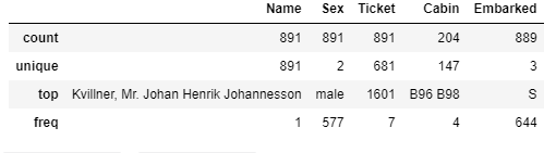
train_df.describe()
|
cs |

--- object describe
--- info

--- > Correlation between The Features
|
1
2
3
4
|
sns.heatmap(data.corr(), annot=True, cmap='RdYlGn', linewidths=0.2)
fig=plt.gcf()
fig.set_size_inches(10,8)
plt.show()
|
cs |

Filling NaN
|
1
2
3
4
|
sns.heatmap(data.corr(), annot=True, cmap='RdYlGn', linewidths=0.2)
fig=plt.gcf()
fig.set_size_inches(10,8)
plt.show()
|
cs |
Pivoting
1 |
train_df[['Pclass', 'Survived']].groupby(['Pclass'],as_index=False).mean().sort_values(by='Survived', ascending=False)
|
cs |
Visualizing

---> Distritution by class
|
1
2
3
4
|
# grid = sns.FacetGrid(train_df, col='Pclass', hue='Survived')
grid = sns.FacetGrid(train_df, col='Survived', row='Pclass', size=2.2, aspect=1.6)
grid.map(plt.hist, 'Age', alpha=.5, bins=20)
grid.add_legend();
|
cs |

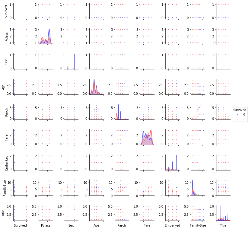
KDE
|
1
2
3
|
g = sns.pairplot(train[[u'Survived', u'Pclass', u'Sex', u'Age', u'Parch', u'Fare', u'Embarked',
u'FamilySize', u'Title']], hue='Survived', palette = 'seismic',size=1.2,diag_kind = 'kde',diag_kws=dict(shade=True),plot_kws=dict(s=10) )
g.set(xticklabels=[])
|
cs |
'데이터분석' 카테고리의 다른 글
| DB Oracle SQL 구문 (0) | 2020.07.13 |
|---|---|
| t-distribution (0) | 2020.06.14 |
| 공공부문 (0) | 2020.06.10 |
| [차원축소][PCA의 원리] Principal component analysis (0) | 2020.02.06 |
| bartlett.test 등분산 검정 (0) | 2019.12.19 |