[Remark] All the probability metrics we need.

---

All the probability metrics we need

 This post explains the probability metrics, including only the essential parts of the them. 

• Kullback-Leiber
• Total variation
• Kolmogorov-Smirnov
• Wasserstein
• Maximum mean discrepancy

---

Kullback-Leiber

Consider two probability distributions $P$ and $Q$. The Kullback-Leiber Distance is defined by 

 

$$\begin{aligned}KL(P||Q) &= \sum_x P(x) \log \frac{P(x)}{Q(x)} \\ KL(P||Q) &= (-\sum_x P(x)\log Q(x)) - (-\sum_x P(x)\log P(x)) \\&= H(P,Q) - H(P)\end{aligned}$$

 

Two equations are same, the second one shows the relationship between KL divegence and entropy. KL is the difference of two entropies, the relative entropy $H(P,Q)$ and $H(P)$. Note that $H(P,Q) \ge H(P)$ holds for all $Q$ and therefore, $KL(P||Q)$ is always positive. 

 

Remark

The first case: there is an x such that two probabilities are zero. The second and the third cases are describes cases when one of two distributions has x such that the probability of x is zero. 

Note that there are three possible zeros for the equation and the last case has an infinity value

• $0 \log \frac{0}{0} = 0$ # $p(x) = 0$ and $q(x) = 0$     # valid value 
• $0 \log \frac{0}{q(x)} = 0$ # $p(x) = 0$ and $q(x) \ne 0$.     # valid value 
• $p(x) \log \frac{p(x)}{0} = \infty$ # $p(x) \ne 0$ and $q(x) = 0$.   # invalid value

 

Therefore, it is required that $P(x) >0$ implies $Q(x) >0$. Also, there is an example, when KL becomes infinity when two distributions have the same support. see also  here

---

Total Variation

Consider two probability measures $P$ and $Q$. Total variation distance of probability measures

 

# a set of support perspective

$$TV(P, Q) = \sup_{A\in \mathcal{F}} P(A) - Q(A).$$ 

# all support perspective

$$TV(P, Q) = \frac{1}{2} \sum_ x |P(x) - Q(x) |$$ 

The red parts are the summation of the differences (all support perspective)

Remark

• The first definition multiply 1/2 because the maximum value of summation is 2.
• $TV(P,Q) \ge P(A) - Q(A)$ for $\forall A \in \mathcal{F}$ holds. Therefore $TV(\cdot, \cdot)$ is the largest possible difference between the probabilities $P$ and $Q$ that $P$ and $Q$ can assign to the same event.

Example

Consider the following example

Consider three types of supports. We calculate the difference of the probabilities on each support. 

• $P(A_1 ) - Q(A_1 ) = 1 - 0 = 1$
• $P(A_2 ) - Q(A_2) = 1 - 1 = 0$
• $TV(P,Q) = \sup_{A\in \mathcal{F}} P(A) - Q(A) = 1$
• $TV(P,Q) = \frac{1}{2} \sum_x |P(x) - Q(x) | = \frac{1}{2} \sum_{x\in A_1} |P(x) - 0| + \frac{1}{2} \sum_{x\in A_3}|0 - Q(x)| = 1$

 

Note that when the supports for two distributions are disjoint, $TV(P,Q) = 1$ holds for all $P$ and $Q$.

---

Kolmogorov-Smirnov

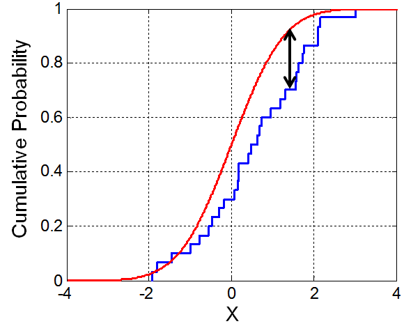
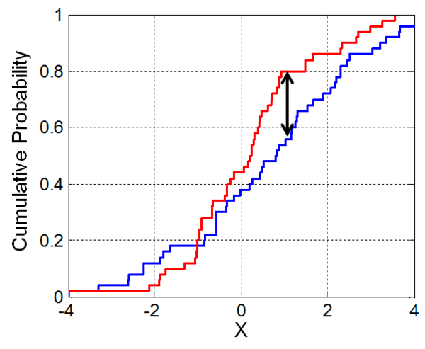
The Kolmogorov-Smirnov statistic quantifies a distance between the empirical distribution function of the sample and the cumulative distance function of the reference distribution, or between the empirical distribution functions of two samples.

• The empirical distribution function $F_n$ for $n$ independent and identical distributed ordered observation $X_i$
• $F_n(x) = \frac{\text{number of (elements in the sample }\le x)}{n}= \frac{1}{n} \sum_{i=1}^n \mathbb{1}_{(-\infty, x]} (X_i)$

 

Kolmogorov-Smirnov statistic for a given cumulative distribution function $F(x)$ is

$$D_n = \sup_x |F_n(x) - F(x)|$$

 

Kolmogorov-Smirnov distance measures the supremum distance of c.d.f for each $x$.

 

One sample ↔ distribution (note that the red curve is the distribution) / Two samples (note that the red curve is a step function) soucre: wikipedia, Kolmogorov-Smirnov

 

Remark

Kolmogorov-Smirnov distance requires similar support

---

Wasserstein Distance

Assume that we have $f$ and want to transport it to $g$ and $h$ each. Which one has a less cost? Obviously moving $f$ to $g$ has a less cost. The Wasserstein distance calculate such a degree for given two distributions.

We want to move f to g or f to h. Obviously moving f to h must have larger cost.

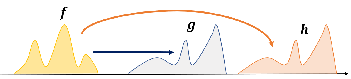
Wassertstein distance is also called earth mover’s distance. Asuume that, there are two functions f and g.

• using function distances, $||f - g ||_\infty \approx ||f- h ||_\infty$
• using the Wasserstein distance, $d_{w_1} (f,g) < d_{w_1} (f,.h)$

 

Formal

Consider the set of possible couplings $\Pi(v, \mu)$ between probability measures $v$ and $\mu$.

$\Pi(v,\mu)$ contains all possible distributions $\pi$ on $\mathcal{Z} \times \mathcal{Z}$ such that if $(Z,Z') \sim \pi$ then $Z \sim v$ and $Z \sim u$.

p-Wasserstein distance is

$$W_p (v, \mu) = \Big( \inf_{\pi \in \Pi(v,\mu) } \int ||z-z'||^p d\pi(z,z') \Big)^{1/p}$$

Remark

Here $\pi$ is a transport policy from $Z$ to $Z'$ and we want to minimize cost $||Z-Z'||^p$

Examples

• Point masses: for given $\mu_1 = \delta_{a_1}, \text{ } \mu_2 = \delta_{a_2}$ be two Dirac delta distributions located at points $a_1$ and $a_2$ in $\mathbb{R}$. the $p$-Wasserstein distance $d_{w_p} (\mu_1, \mu_2)$ is $d_{w_p} = |a_1 - a_2|$
• Normal distributions: for given $\mu_1 = \mathcal{N}(m_1, C_1)$ and $\mu_2 = \mathcal{N}(m_2, C_2)$ , the 2-Wasserstein distrnace $d_{w_2} (\mu_1, \mu_2)$ can be computedwhere $m_i \in \mathbb{R}^n , C_i \in \mathbb{R}^{n\times n}$
• $d_{w_2} (\mu_1, \mu_2)^2 = ||m_1 - m_2||^2 + \text{trace} (C_1 + C_2 - 2 (C_2^{1/2} C_1 C_2^{1/2})^{1/2})$

---

Maximum mean discrepency

mean discrepency

Consider the following three cases.

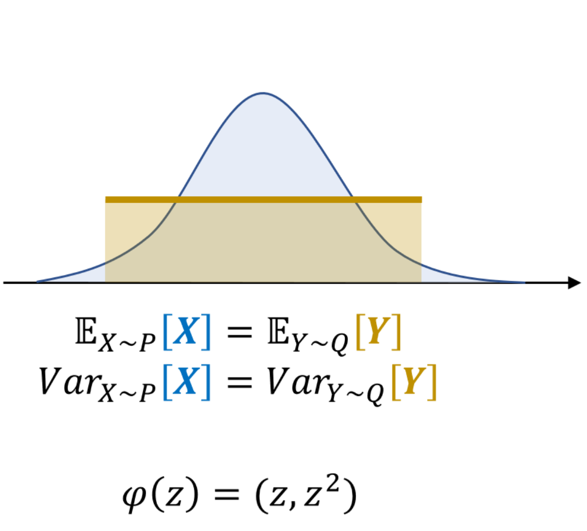
• The first case has two distributions $P$ and $Q$. Even though they are not same the mean is same.
• The second case: the mean and the variance of two distributions are equal, but there is a remaining discrepency.
• The thrid case: every moments of two distributions are equal. In this case two distributions are equal and there is no discrepency. 

The cases where the moments are equal for two distributions. 1) the mean values are equal.  2) the mean values and the variances are equal.   3) all the moments are eqaul. The last case is when two distributions are identical. 

 

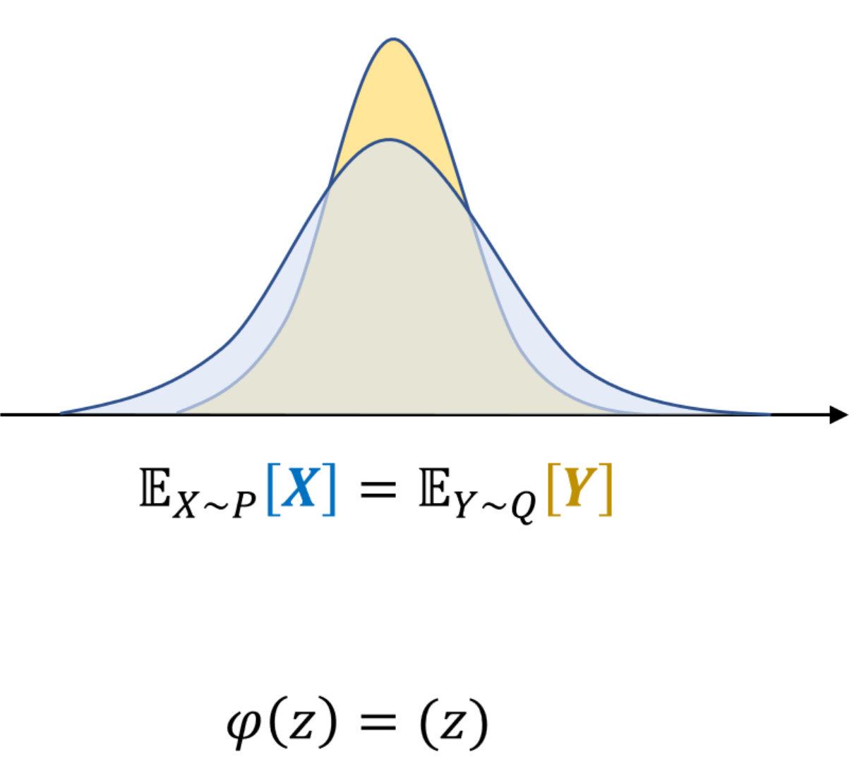
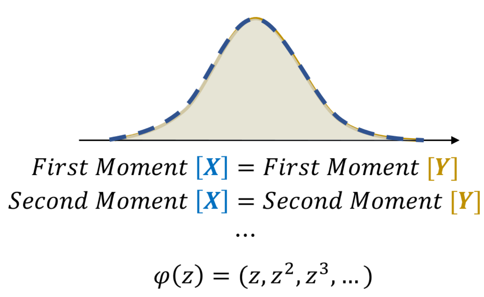
Therefore, it is intuitive that, we may consider all the moments if we want to the calculate the discrepency of two distributions by the mean value of the distribuiton.

Hence, instead of comparing just mean value $d(\mathbb{E}_{X\sim P}[X] , \mathbb{E}_{Y\sim Q}[Y])$ of two distributions, we may comsider all the properties of the variables by calculating $d(\mathbb{E}_{X\sim P}[(X, X^2, X^3 , \cdots )] , \mathbb{E}_{Y\sim Q}[(Y, Y^2, Y^3, \cdots )] )$ which is equal to the case $d(\mathbb{E}_{X\sim P}[\varphi(X)] , \mathbb{E}_{Y\sim Q}[\varphi(Y)] )$ when $\phi(z) = (z, z^2, \cdots)$

 

Formal

Let $P$ and $Q$ be distributions over a set $\mathcal{X}$. The MMD is defined by a feature map $\varphi : \mathcal{X} \rightarrow \mathcal{H}$, where $\mathcal{H}$ is a reproducing kernel Hilbert space.

In general, the MMD is

$$\text{MMD} (P, Q) = || \mathbb{E}_{X\sim P}[\varphi(X)] - \mathbb{E}_{Y\sim Q}[\varphi(Y)]||$$

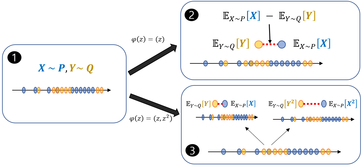
The calculation of MMD assumes the case where we are not able to get a probability density function of the samples and we only have samples. Therefore, we compare two distributions by just samlpes. The sample based mean discrepency can be viewed like this.

Sample based interpretation of the mean discrepency.&nbsp; 1) Given samples distributed by P and Q each.&nbsp; &nbsp;2) Comparing the mean value only.&nbsp; &nbsp;3) comparing the mean values and the variances of the samples.

 

If $\varphi$ maps to a general reproducing kernel Hilbert Space (RKHS), then you can apply kernel trick to compute the MMD. It is known that there are many kernels including the Gaussian kernel, such that lead to the MMD being zero if and only the distributions are identical.

 

Letting $k(x,y) = \langle \varphi(x) , \varphi(y) \rangle_{\mathcal{H}}$

$$\begin{aligned} \text{MMD}(P,Q) &= || \mathbb{E}_{X\sim P} [\varphi(X) ] - \mathbb{E}_{Y\sim Q} [\varphi(Y) ]||\mathcal{H}^2 \ \\& = \langle\mathbb{E}_{X\sim P} [\varphi(X) ], \mathbb{E}_{X'\sim P} [\varphi(X') ]\rangle_\mathcal{H} + \langle \mathbb{E}_{Y\sim Q} [\varphi(Y) ] , \mathbb{E}_{Y'\sim Q} [\varphi(Y) ]\rangle_\mathcal{H} \ \\&~~~~~~~~ -2 \langle \mathbb{E}_{X\sim P} [\varphi(X) ], \mathbb{E}_{Y\sim Q} [\varphi(Y) ]\rangle_\mathcal{H}\ \\&= \mathbb{E}_{X,X'\sim P} [k(X, X') ]+ \mathbb{E}_{Y,Y'\sim Q} [k(Y,Y') ]- 2 \mathbb{E}_{X\sim P, Y\sim Q} [k(X,Y)] \end{aligned}$$

 

Remark

• We have a fixed kernel $k (\cdot,\cdot)$ to compute the MMD.
• We need to compute pairwise data points $(X', X)$, $(Y',Y)$, and $(X,Y)$
• If we use kenrel $k(x,y) = |x-y |$, it is equal to the case which we compare only the mean values of two distribution. (not able to match the vairance. ) * I’m not sure
• We usually use the Gaussian kernel for full expresiveness and we match all the moments of the distribution because $e^x = 1+ x+ \frac{1}{2} x^2 +\cdots$ contains all the moments.

Recommanded article

---

😀 It is wellcome to give me any advice including typos via comments or email bumjin@kaist.ac.kr